Turn on suggestions
Auto-suggest helps you quickly narrow down your search results by suggesting possible matches as you type.
Showing results for
Data Engineering
Turn on suggestions
Auto-suggest helps you quickly narrow down your search results by suggesting possible matches as you type.
Showing results for
- Databricks
- Data Engineering
- Why is execution too fast?
Options
- Subscribe to RSS Feed
- Mark Topic as New
- Mark Topic as Read
- Float this Topic for Current User
- Bookmark
- Subscribe
- Mute
- Printer Friendly Page
Why is execution too fast?
Options
- Mark as New
- Bookmark
- Subscribe
- Mute
- Subscribe to RSS Feed
- Permalink
- Report Inappropriate Content
11-26-2022 04:26 PM
I have a table, full scan of which takes ~20 minutes on my cluster. The table has "Time" TIMESTAMP column and "day" DATE column. The latter is computed (manually) as "Time" truncated to day and used for partitioning.
I query the table using predicate based on "Time" ("day" is not included), but it works too fast (~10 s). I expect that partition skipping is not used. EXPLAIN also shows "PartitionFilters: []", so I assume partitioning cannot account for the performance gain. In fact, adding or removing "day" into predicate does not seem to have any performance impact.
How to explain the the query returning result so fast (~10 s)? What could be other mechanisms that could provide such a performance boost?
Table:
CREATE TABLE myschema.mytable (
  Time TIMESTAMP,
  TagName STRING,
  Value DOUBLE,
  Quality INT,
  day DATE,
  isLate BOOLEAN)
USING delta
PARTITIONED BY (day, isLate)
Query:
select date_trunc("minute", Time) as time, TagName, avg(Value) as value
from myschema.mytable
where Time between current_timestamp() - interval '3 days' and current_timestamp()
group by date_trunc("minute", Time), TagName
Update 1:
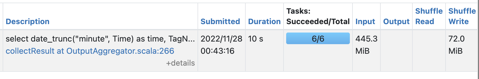
The amount of input it shows for the stage is suspiciously small:


Labels:
- Labels:
-
Date Column
-
Partitioning
-
Performance
12 REPLIES 12
Anonymous
Not applicable
Options
- Mark as New
- Bookmark
- Subscribe
- Mute
- Subscribe to RSS Feed
- Permalink
- Report Inappropriate Content
11-26-2022 10:28 PM
Hi @Vladimir Ryabtsev
Great to meet you, and thanks for your question!
Let's see if your peers in the community have an answer to your question first. Or else bricksters will get back to you soon.
Thanks
Options
- Mark as New
- Bookmark
- Subscribe
- Mute
- Subscribe to RSS Feed
- Permalink
- Report Inappropriate Content
11-27-2022 06:40 AM
Hi @Vladimir Ryabtsev ,
Because you are creating a delta table, I think that you are seeing a performance improvement because of Dynamic Partition pruning,
According to the documentation, "Partition pruning can take place at query compilation time when queries include an explicit literal predicate on the partition key column or it can take place at runtime via Dynamic Partition Pruning." Also do read these documentations if it helps. https://www.databricks.com/blog/2020/04/30/faster-sql-queries-on-delta-lake-with-dynamic-file-prunin...
If you want to test it out, turn off the DFP using spark.databricks.optimizer.dynamicFilePruning by setting it to false and check if the performance is still the same.
If not, it would be great if you posted the DAG so that we can take a look at what is happening.
Hope this helps...Cheers.
Options
- Mark as New
- Bookmark
- Subscribe
- Mute
- Subscribe to RSS Feed
- Permalink
- Report Inappropriate Content
11-27-2022 04:36 PM
@Uma Maheswara Rao Desula your documentation states the following criteria for DFP to be used:
- The inner table (probe side) being joined is in Delta Lake format
- The join type is INNER or LEFT-SEMI
- The join strategy is BROADCAST HASH JOIN
- The number of files in the inner table is greater than the value for spark.databricks.optimizer.deltaTableFilesThreshold
In my case, the query does not even have any joins.
Anyway I tried switching off the parameter you gave and it did not make any difference.
Options
- Mark as New
- Bookmark
- Subscribe
- Mute
- Subscribe to RSS Feed
- Permalink
- Report Inappropriate Content
11-27-2022 09:48 PM
Hi @Vladimir Ryabtsev
Need some more info
- Can you get the total size & number of records the of delta table you have ?
- "full scan of which takes ~20 minutes on my cluster" - are you using the same cluster for query and if yes, the screenshot of that full scan too.
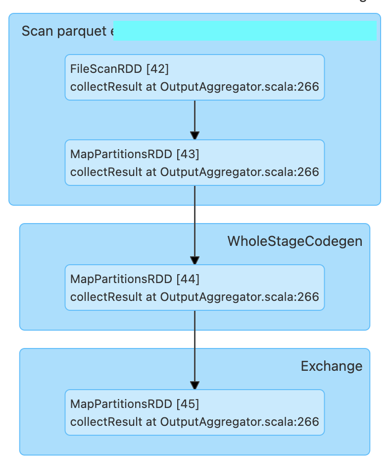
- For the DAG, after you click on Job details in the spark UI, you will find a highlighted id for the associated SQL query at the top. Click on that id, expand all the details in the query plan visualization and kindly paste it here.
To find the size of a delta table, you can use a Apache Spark SQL command.
import com.databricks.sql.transaction.tahoe._
val deltaLog = DeltaLog.forTable(spark, "dbfs:/<path-to-delta-table>")
val snapshot = deltaLog.snapshot // the current delta table snapshot
println(s"Total file size (bytes): ${deltaLog.snapshot.sizeInBytes}")
Options
- Mark as New
- Bookmark
- Subscribe
- Mute
- Subscribe to RSS Feed
- Permalink
- Report Inappropriate Content
11-29-2022 03:02 PM
- I could not run your snippet because Scala is disallowed on the cluster, but DESC DETAIL shows 233 GiB in 4915 files. When launched without filter predicate, the biggest job shows input of size 105 GiB. Rows count: 23.5 B.
- The same cluster was used for the comparison, as comparing performance with a cluster of different size would be meaningless.
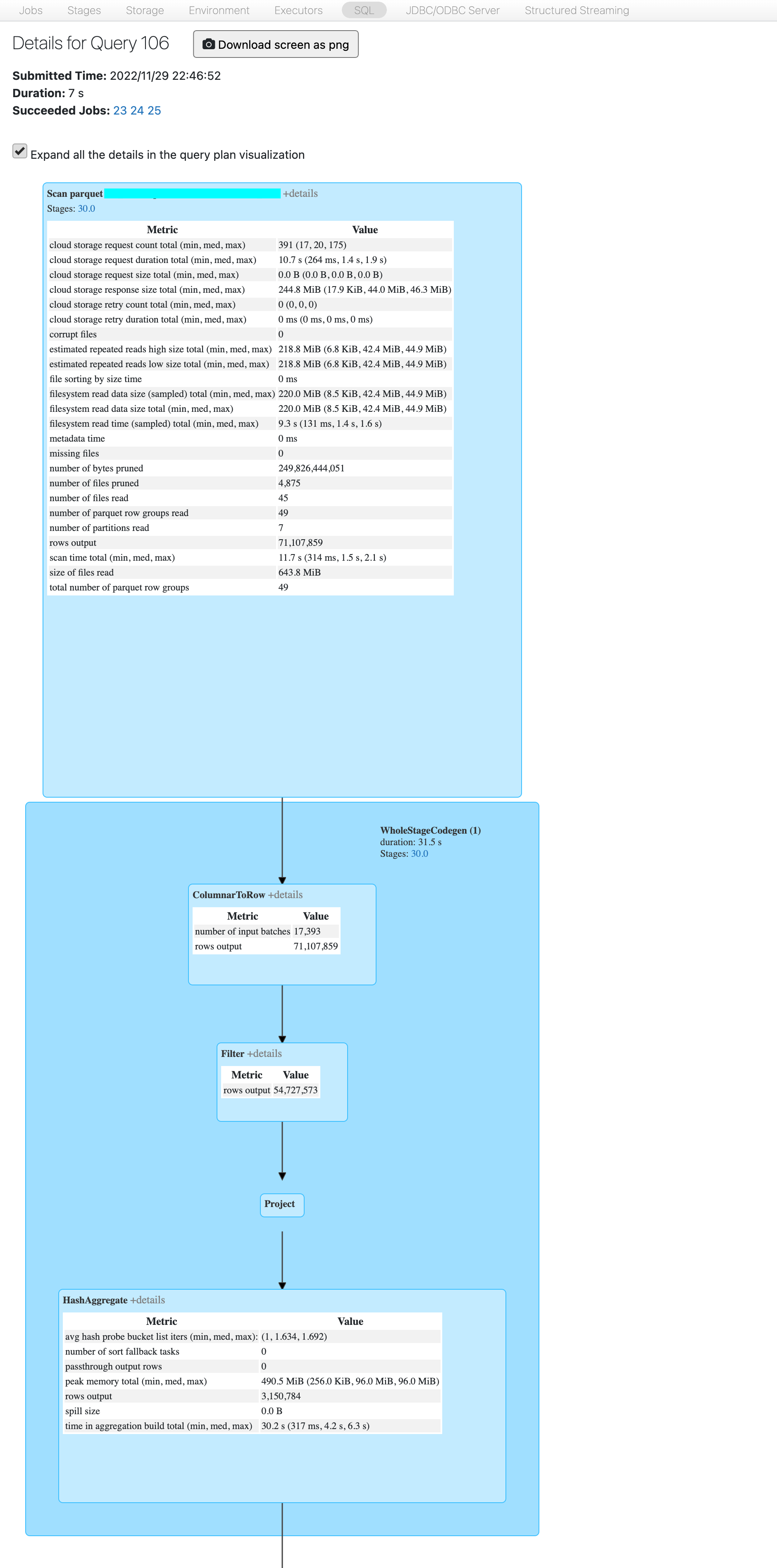
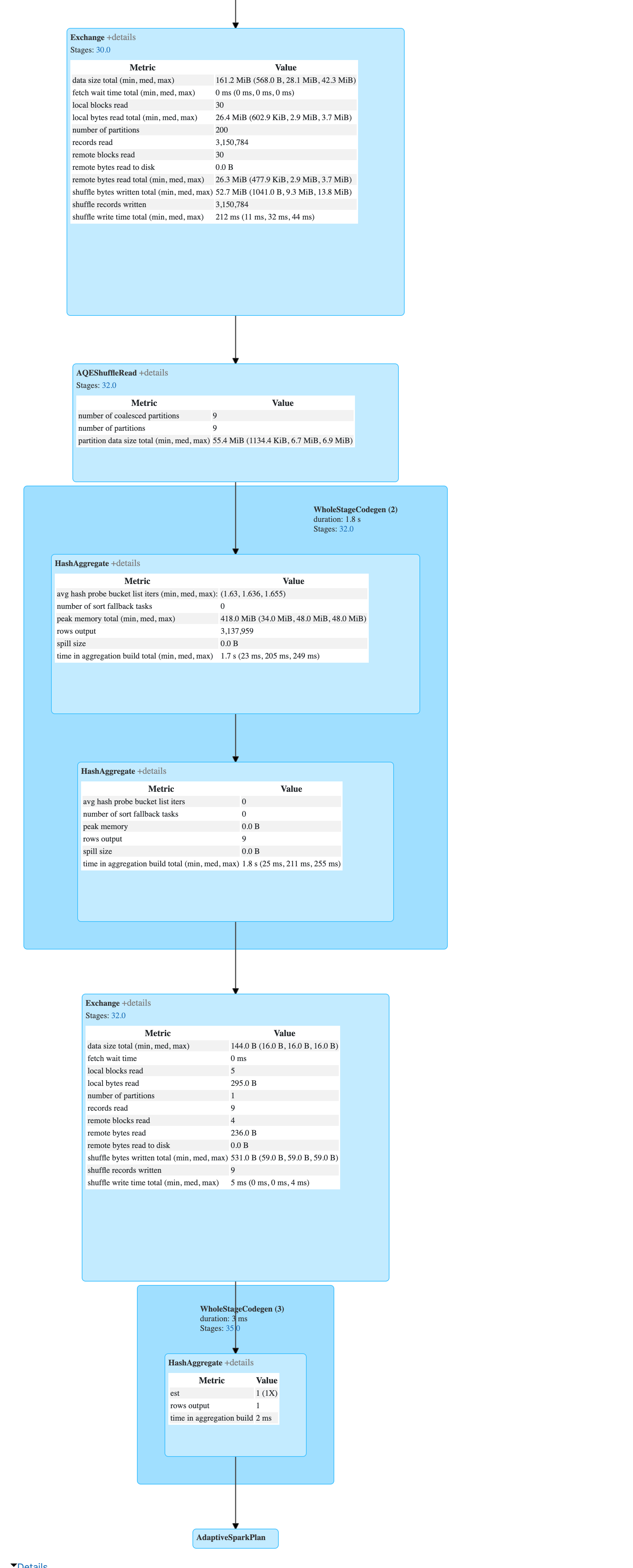
- Please validate the data below:


== Physical Plan ==
AdaptiveSparkPlan (22)
+- == Final Plan ==
   * HashAggregate (13)
   +- ShuffleQueryStage (12), Statistics(sizeInBytes=144.0 B, rowCount=9, isRuntime=true)
      +- Exchange (11)
         +- * HashAggregate (10)
            +- * HashAggregate (9)
               +- AQEShuffleRead (8)
                  +- ShuffleQueryStage (7), Statistics(sizeInBytes=161.2 MiB, rowCount=3.15E+6, isRuntime=true)
                     +- Exchange (6)
                        +- * HashAggregate (5)
                           +- * Project (4)
                              +- * Filter (3)
                                 +- * ColumnarToRow (2)
                                    +- Scan parquet ccc.sss.ttt (1)
+- == Initial Plan ==
   HashAggregate (21)
   +- Exchange (20)
      +- HashAggregate (19)
         +- HashAggregate (18)
            +- Exchange (17)
               +- HashAggregate (16)
                  +- Project (15)
                     +- Filter (14)
                        +- Scan parquet ccc.sss.ttt (1)


(1) Scan parquet ccc.sss.ttt
Output [4]: [Time#2824, TagName#2825, day#2831, isLate#2832]
Batched: true
Location: PreparedDeltaFileIndex [mcfs-abfss://t-125a3c9d-90a3-46dc-a577-196577aff13d+concon@sasasa.dfs.core.windows.net/tttddd/delta]
PushedFilters: [IsNotNull(Time), GreaterThanOrEqual(Time,2022-11-26 22:46:52.42), LessThanOrEqual(Time,2022-11-29 22:46:52.42)]
ReadSchema: struct<Time:timestamp,TagName:string>

(2) ColumnarToRow [codegen id : 1]
Input [4]: [Time#2824, TagName#2825, day#2831, isLate#2832]

(3) Filter [codegen id : 1]
Input [4]: [Time#2824, TagName#2825, day#2831, isLate#2832]
Condition : ((isnotnull(Time#2824) AND (Time#2824 >= 2022-11-26 22:46:52.42)) AND (Time#2824 <= 2022-11-29 22:46:52.42))

(4) Project [codegen id : 1]
Output [2]: [TagName#2825, date_trunc(minute, Time#2824, Some(Etc/UTC)) AS _groupingexpression#2839]
Input [4]: [Time#2824, TagName#2825, day#2831, isLate#2832]

(5) HashAggregate [codegen id : 1]
Input [2]: [TagName#2825, _groupingexpression#2839]
Keys [2]: [_groupingexpression#2839, TagName#2825]
Functions: []
Aggregate Attributes: []
Results [2]: [_groupingexpression#2839, TagName#2825]

(6) Exchange
Input [2]: [_groupingexpression#2839, TagName#2825]
Arguments: hashpartitioning(_groupingexpression#2839, TagName#2825, 200), ENSURE_REQUIREMENTS, [id=#2040]

(7) ShuffleQueryStage
Output [2]: [_groupingexpression#2839, TagName#2825]
Arguments: 0, Statistics(sizeInBytes=161.2 MiB, rowCount=3.15E+6, isRuntime=true)

(8) AQEShuffleRead
Input [2]: [_groupingexpression#2839, TagName#2825]
Arguments: coalesced

(9) HashAggregate [codegen id : 2]
Input [2]: [_groupingexpression#2839, TagName#2825]
Keys [2]: [_groupingexpression#2839, TagName#2825]
Functions: []
Aggregate Attributes: []
Results: []

(10) HashAggregate [codegen id : 2]
Input: []
Keys: []
Functions [1]: [partial_count(1) AS count#2841L]
Aggregate Attributes [1]: [count#2840L]
Results [1]: [count#2841L]

(11) Exchange
Input [1]: [count#2841L]
Arguments: SinglePartition, ENSURE_REQUIREMENTS, [id=#2093]

(12) ShuffleQueryStage
Output [1]: [count#2841L]
Arguments: 1, Statistics(sizeInBytes=144.0 B, rowCount=9, isRuntime=true)

(13) HashAggregate [codegen id : 3]
Input [1]: [count#2841L]
Keys: []
Functions [1]: [finalmerge_count(merge count#2841L) AS count(1)#2833L]
Aggregate Attributes [1]: [count(1)#2833L]
Results [1]: [count(1)#2833L AS count(1)#2836L]

(14) Filter
Input [4]: [Time#2824, TagName#2825, day#2831, isLate#2832]
Condition : ((isnotnull(Time#2824) AND (Time#2824 >= 2022-11-26 22:46:52.42)) AND (Time#2824 <= 2022-11-29 22:46:52.42))

(15) Project
Output [2]: [TagName#2825, date_trunc(minute, Time#2824, Some(Etc/UTC)) AS _groupingexpression#2839]
Input [4]: [Time#2824, TagName#2825, day#2831, isLate#2832]

(16) HashAggregate
Input [2]: [TagName#2825, _groupingexpression#2839]
Keys [2]: [_groupingexpression#2839, TagName#2825]
Functions: []
Aggregate Attributes: []
Results [2]: [_groupingexpression#2839, TagName#2825]

(17) Exchange
Input [2]: [_groupingexpression#2839, TagName#2825]
Arguments: hashpartitioning(_groupingexpression#2839, TagName#2825, 200), ENSURE_REQUIREMENTS, [id=#1937]

(18) HashAggregate
Input [2]: [_groupingexpression#2839, TagName#2825]
Keys [2]: [_groupingexpression#2839, TagName#2825]
Functions: []
Aggregate Attributes: []
Results: []

(19) HashAggregate
Input: []
Keys: []
Functions [1]: [partial_count(1) AS count#2841L]
Aggregate Attributes [1]: [count#2840L]
Results [1]: [count#2841L]

(20) Exchange
Input [1]: [count#2841L]
Arguments: SinglePartition, ENSURE_REQUIREMENTS, [id=#1941]

(21) HashAggregate
Input [1]: [count#2841L]
Keys: []
Functions [1]: [finalmerge_count(merge count#2841L) AS count(1)#2833L]
Aggregate Attributes [1]: [count(1)#2833L]
Results [1]: [count(1)#2833L AS count(1)#2836L]

(22) AdaptiveSparkPlan
Output [1]: [count(1)#2836L]
Arguments: isFinalPlan=true
Is that what you are asking about? Please let me know if I can provide more information.
Options
- Mark as New
- Bookmark
- Subscribe
- Mute
- Subscribe to RSS Feed
- Permalink
- Report Inappropriate Content
12-02-2022 10:24 AM
Hi @Vladimir Ryabtsev
It looks like it is actually the performance obtained by pruning.
As an answer to your previous query, I was not referring to the DFP based on joins. I was referring to the pruning by literal filters. I just used a common term DFP as I don't exactly remember what type of pruning they call this (filter pruning maybe lol).
Do check out this blog I found in my old bookmarks for further info.
Cheers..
Options
- Mark as New
- Bookmark
- Subscribe
- Mute
- Subscribe to RSS Feed
- Permalink
- Report Inappropriate Content
12-02-2022 11:31 AM
Hi @Uma Maheswara Rao Desula,
This is the same link you shared previously. This article says about inferring partition predicate from a joined dictionary table. In such a case the predicate is not mentioned in the query, but it can inferred according to the query logic (this is why it is called dynamic). The optimizer understands that the JOIN predicate is equal (or a subset) of partitioning predicate, so it can utilize partitioning. As the first step it filters the dictionary table to find the values that contribute to JOIN. When done, it used partition pruning based on values from the first step. Exact partitions cannot be identified prior to execution (those depend on the content in the dictionary table), so the dynamic style. Same partitioning technology, but a bit smarter.
In my case what could be the logic for the engine that it can use to utilize partitioning? "Time" column is not in partitioning predicate, and "day" column is filled manually, so the engine does not have information to convert predicate for "Time" into predicate for "day".
Options
- Mark as New
- Bookmark
- Subscribe
- Mute
- Subscribe to RSS Feed
- Permalink
- Report Inappropriate Content
12-02-2022 12:13 PM
Hi @Vladimir Ryabtsev
Genuinely sorry. I thought there was a partition column used in the query which is causing a partition pruning. Blame my sleepy eyes and mobile screen. 😥
But again, what I was talking about was a simple filter partition pruning which again you can park aside for now.
As for your query, now I can think of only two possible factors for your performance improvement. (I'm already assuming that you are not calling an action on the table you already created by doing a full scan as it delta caches the data).
- Columnar Projection : Columnar data formats use this feature where it reads only the data for the columns in the query and skips the rest. So, the lesser data linked to other columns, the more performance you obtain. In your case, it does not need to read all the data of the columns but just read a subset of it. So spark optimizes the IO path and the amount of data read from storage will be a lot less. This part I think will be in the Project field of the physical plan where you will be able to find only the columns it reads.
- Predicate PushDown - There will be some performance improvement because of PP as again the amount of data to be read gets reduced because of this. So spark calculates the filters against the metadata and it can skip performing I/O on data altogether which it decides is not needed. This again reduces the workload.
There were some testing done on these use cases to check out the performance gains. You will actually find some numbers to reinforce your query. I don't exactly remember the blog author but I reckon his name will be like carnal or canal something. Will scrim through my old bookmarks and attach it here in case I find it. Till then try to analyse for the above two possibilities.
It really was a wonderful discussion.
Cheers..
Options
- Mark as New
- Bookmark
- Subscribe
- Mute
- Subscribe to RSS Feed
- Permalink
- Report Inappropriate Content
12-02-2022 05:45 PM
Please don't be sorry, I appreciate your willingness to help!
Yes, the performance I have is in the "cold" state, no full scans prior that (and actually it does not have big impact in my case, filtered scan after full scan is not faster than cold one, I think because it cannot cache that much data anyway).
- Well, somewhat, probably... There are some traces of that in the plan, but: there are at least 3 columns involved in the query: Time (8 bytes), TagName (~25 bytes), Value (8 bytes). The ones that can be skipped: Quality (4 bytes), day (4 bytes), isLate (1 bit). This gives approximately 20% of data that can be skipped. But the stats show that the skipped part is ~99.5%.
- Push Down works similarly to DFP, transferring query predicate to individual relation predicates. In my case there's just one table, no need to push, the filter is already final (and we see that in the plan).
I understand that it looks like I criticize every your assumption, but I really think those assumptions cannot explain such a boost so far. It looks like we are missing a huge chunk of optimization feature, and I'd like to understand what it is, because if we can learn how to use it on purpose, it can provide a huge performance benefit.
I am thinking, is it possible to get the plan detailed to individual parquet files? My idea is that if I find out that the list of files is limited to directories representing 3 latest days only, we can finally make the conclusion whether partitioning is involved or not.
Options
- Mark as New
- Bookmark
- Subscribe
- Mute
- Subscribe to RSS Feed
- Permalink
- Report Inappropriate Content
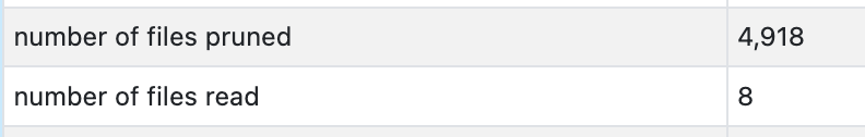
12-02-2022 06:02 PM
To develop more on point #1, even on a simple query like "select count(Time) from mytable where Time between '2018-11-27' and '2018-11-30'" with a short Time interval, the number of read files is consistently small and number of pruned files is consistently big.

Options
- Mark as New
- Bookmark
- Subscribe
- Mute
- Subscribe to RSS Feed
- Permalink
- Report Inappropriate Content
12-02-2022 07:31 PM
I think I found it: https://stackoverflow.com/a/57891876/947012
This can explain the performance as, thanks to partitioning, most files can be skipped based on parquet metadata. Partitioning is not used as a feature, but contributes into organization of data into separate files.
That's my theory... Still interested in confirming. I wonder if it is realistic that it reads footers of ~5000 files in under 5 seconds to achieve that skipping.
Options
- Mark as New
- Bookmark
- Subscribe
- Mute
- Subscribe to RSS Feed
- Permalink
- Report Inappropriate Content
11-29-2022 03:06 AM
Hi @Vladimir Ryabtsev, We haven’t heard from you since the last response from @Uma Maheswara Rao Desula, and I was checking back to see if their suggestions helped you.
Or else, If you have any solution, please share it with the community, as it can be helpful to others.
Also, Please don't forget to click on the "Select As Best" button whenever the information provided helps resolve your question.
Announcements


Welcome to Databricks Community: Lets learn, network and celebrate together
Join our fast-growing data practitioner and expert community of 80K+ members, ready to discover, help and collaborate together while making meaningful connections.
Click here to register and join today!
Engage in exciting technical discussions, join a group with your peers and meet our Featured Members.
Related Content
- Proper way to collect Statement ID from JDBC Connection in Administration & Architecture
- I have to run the notebook in concurrently using process pool executor in python in Data Engineering
- Pyspark execution error in Data Engineering
- Trying to run databricks academy labs, but execution fails due to method to clearcache not whilelist in Data Engineering
- Why is Dlt pipeline processing streaming data so slow? in Data Engineering