Turn on suggestions
Auto-suggest helps you quickly narrow down your search results by suggesting possible matches as you type.
Showing results for
Technical Blog
Explore in-depth articles, tutorials, and insights on data analytics and machine learning in the Databricks Technical Blog. Stay updated on industry trends, best practices, and advanced techniques.
Turn on suggestions
Auto-suggest helps you quickly narrow down your search results by suggesting possible matches as you type.
Showing results for
- Databricks Community
- Technical Blog
- Introducing the DeepSpeed Distributor on Databrick...
Databricks Employee
Options
- Subscribe to RSS Feed
- Mark as New
- Mark as Read
- Bookmark
- Subscribe
- Printer Friendly Page
- Report Inappropriate Content
02-12-2024
07:00 AM

Table of Contents
Overcoming GPU bottlenecks
The major bottleneck in deep learning training today is the amount of RAM per GPU - they simply don’t have a lot of it.
|
GPU Model |
VRAM (GB) |
AWS |
Azure |
|
T4 |
16 |
g4dn |
NCasT4_v3 |
|
V100 |
16 |
p3 |
NC_v3 |
|
V100 |
32 |
p3dn |
NDv2 |
|
A10 |
24 |
g5 |
NVadsA10_v5 |
|
A100 |
40 |
p4d |
NDasrA100_v4 |
|
A100 |
80 |
p4de |
NDm_A100_v4 |
|
H100 |
80 |
p5 |
NDm_H100_v5 |
Common GPUs - their instance types and available RAM
To address this issue, two main paradigms have emerged: data parallel and model parallel training.
Data parallel training involves splitting the data across multiple GPUs. In this scenario, each GPU needs to contain a full copy of the model and training artifacts (the optimizer state and gradients), greatly reducing available RAM for training data.

On the other hand, model parallel training splits the model itself across multiple GPUs, freeing up RAM on each machine. In this scenario a new bottleneck appears - the available network bandwidth between the distributed GPUs.
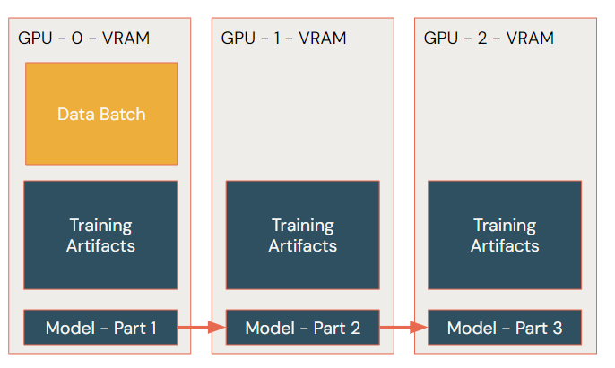
In the model parallel paradigm, the memory efficiency of DeepSpeed can be leveraged to allow us to train larger models without incurring exorbitant costs.
Understanding DeepSpeed and the DeepSpeed Distributor
The DeepSpeed library consists of three key modules: the training of, inference with and compression of deep learning models. In this article we focus on model training.
To understand how DeepSpeed fits and how to configure it, we must first unpack the training process. There are two constraints when training large language models and their computer vision cousins: the input / output speeds for loading training data and the amount of memory available per GPU card. For data loading optimizations, refer to our collaboration with Hugging Face and the Torchdelta extension.
For model training, there are three main memory hogs: the model and its weights, the optimizer state and gradients, and the size of the training data. To reduce training time, we want to maximize the amount of data we load on the GPU. This requires configuring DeepSpeed to limit the RAM footprint of the model, optimizer and gradients. Let’s walk through those settings now.
Model Precision Settings
To ensure a high quality chat experience for end users of our LLM applications we want to use the largest models we can. By default, model weights are stored as 32-bit floating point, so even 7 billion parameter models take up all the RAM on smaller GPUs and a considerable chunk on larger ones. DeepSpeed includes optimizations that allow us to train at 16-bit floating point instead, greatly reducing model size. When using 16-bit floating point precision, a good rule of thumb is that an average model requires approximately 2x its number of parameters (billions) in GPU RAM (GB) rather than 4x with the default fp32. Whilst it is possible to use lower precision, these techniques are still more experimental.
There are two types of 16-bit precision to choose from: the normal fp16 and bfloat16. When working with newer Nvidia GPUs (A10/A100/H100) it is recommended to use bfloat16, which can be set as follows in the JSON config file.
"bf16": {
   "enabled": true
}
-
Older GPUs do not support bfloat16 and hence we will fallback to the older less efficient fp16 format, shown below.
"fp16": {
        "enabled": "auto",
        "loss_scale": 0,
        "loss_scale_window": 1000,
        "initial_scale_power": 16,
        "hysteresis": 2,
        "min_loss_scale": 1
    }
We recommend using bfloat compatible GPUs where possible. It has been noted that fp16 training can be unstable and may require manual intervention during the training to change learning rates and avoid NaN losses which is partially why fp16 also has so many additional settings.; For more details check the documentation and Nvidia's guide on mixed precision training
Optimizer and Gradient Settings
The next area that we can look for memory savings is with the optimizer and gradient calculations. This can be done through leveraging the Zero Redundancy Optimizer (ZeRO) settings. ZeRO is the core of DeepSpeed and was first introduced in the research paper. The authors noted that a lot of the weights, states and gradients stored during training are redundant, allowing for them to be partitioned across GPUs and even onto CPU and disk. This does result in the need to move data around and increases network traffic, but the savings in GPU RAM are worth it.
ZeRO has three settings:
- Stage 1: Optimizer State Partitioning
- Stage 2: Optimizer and Gradient Partitioning
- Stage 3: Optimizer, Gradient and Parameter Partitioning
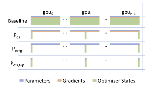
Beyond stage 3 we can also offload calculations onto the CPU and attached storage, though this can come with hefty performance constraints. For an understanding of the possible space savings, see the below diagram from the original ZeRO paper where Stage 1 = Pos, Stage 2 = Pos+g and Stage 3 = Pos+g+p.
As we go from Stages 1 to 3, we can see that we get more and more VRAM savings. Whilst the formulas for calculating VRAM consumption are a little complex, here is a visualization of estimated VRAM requirements per GPU.
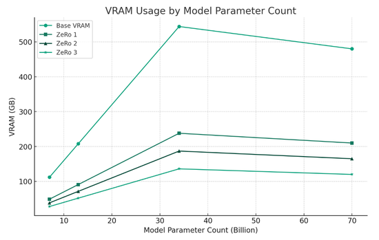
|
Model Parameter Count (B) |
Base VRAM (GB) |
ZeRo 1 (GB) |
ZeRo 2 (GB) |
ZeRo 3 (GB) |
|
7 |
112 |
49 |
38.5 |
28 |
|
13 |
208 |
91 |
71.5 |
52 |
|
34 |
544 |
238 |
187 |
136 |
|
70 |
480 |
210 |
165 |
120 |
Beyond ZeRo 3, it is also possible to offload the optimizer states, gradients and parameters into either CPU RAM or attached NVMe drives. Whilst offload will cause a performance hit, it can allow small setups to train much larger models.
- Offload can be set in the JSON configuration:
# cpu offload
"offload_optimizer": {"device": "cpu"},
"offload_param": {"device": "cpu"},
# gpu offload "offload_optimizer": {"device": "nvme", "nvme_path": "/local_disk0/optimizer"}, "offload_param": {"device": "nvme", "nvme_path": "/local_disk0/param"}
On Databricks clusters, /local_disk0 is the mount path for direct attached storage that you can use as a temporary cache. Offload also requires the installation of libaio-dev, an OS-level library that will require installing via init script (AWS/Azure). When using offload, it is important to make sure that there is sufficient CPU RAM and NVMe storage. It is recommended to set the autoscale local storage setting when creating your cluster if you will use NVMe storage.
How to trigger a DeepSpeed training job
Now that we understand the workings of key DeepSpeed configs, we can look at how to code and launch our pipelines. The beauty of the design around the DeepSpeed Distributor is that it doesn't require extensive code changes in order to leverage it within your workflows. Just like the TorchDistributor, the DeepSpeed flavor can be utilized in two ways:
- Trigger a function written within the existing notebook context
- Trigger an external Python script
Triggering a function from notebooks
In this example, we assume that the training function is called train and it accepts the arguments training_arguments and dataset.
- Running on single node:
from pyspark.ml.deepspeed.deepspeed_distributor import DeepspeedTorchDistributor distributor = DeepspeedTorchDistributor(numGpus=1, nnodes=1, localMode=True, useGpu=True, deepspeedConfig = deepspeed_dict) completed_trainer = distributor.run(train, training_arguments, dataset) -
Running in distributed fashion:
from pyspark.ml.deepspeed.deepspeed_distributor import DeepspeedTorchDistributor

distributor = DeepspeedTorchDistributor(numGpus=4, nnodes=2, localMode=True,
                                        useGpu=True,
deepspeedConfig = deepspeed_dict)

completed_trainer = distributor.run(train, training_arguments, dataset)
To elaborate on the parameters available to DeepSpeedTorchDistributor:
- numGpus: number of GPUs per node
- nnodes: number of nodes to train on
- localMode: if True, trains on the driver node only (for single node cluster) if False will train on the workers
- useGpu: whether to train using GPUs
- deepspeedConfig: JSON file with all configuration parameters
While useGPU is available, it is worth mentioning that DeepSpeed should ideally be used with GPUs.
Triggering a Python script
In addition to executing a train function defined in a notebook, it is possible to use DeepspeedTorchDistributor to load and execute a training script by specifying the path to the Python file and passing command line arguments to it.
- Running on single node:
from pyspark.ml.deepspeed.deepspeed_distributor import DeepspeedTorchDistributor distributor = DeepspeedTorchDistributor(numGpus=4, nnodes=1, localMode=False, useGpu=True, deepspeedConfig = deepspeed_dict) completed_trainer = distributor.run('<path_to_file>/train.py', "--var1 value1", "--var2 value2") - Running in distributed fashion:
from pyspark.ml.deepspeed.deepspeed_distributor import DeepspeedTorchDistributor

distributor = DeepspeedTorchDistributor(numGpus=4, nnodes=2, localMode=False,
                                        useGpu=True,
deepspeedConfig = deepspeed_dict)

completed_trainer = distributor.run('<path_to_file>/train.py', "--var1 value1", "--var2 value2")
Tricks and Tips to be productive
Now that you understand the key DeepSpeed configs and how to launch your training job, we will cover some other considerations that you should be aware of to ensure the smoothest possible experience.
Estimating Memory Requirements
Managing and understanding the requirements to fine tune a particular model can be hard. There are a few helpful rules of thumb first to assess the viability of our training job before consuming any GPU resources.
As discussed, the number of parameters in a model will dictate the amount of VRAM it and its training states will take. If we are training with fp16 or bfloat16 we can use a simple formula:
2 X number of params (B) = VRAM required (GB)
Thus, a 7 billion parameter model like llama_v2_7b will take approximately 14GB VRAM to load in bfloat16 format.
Next, we need to factor in the type of fine-tuning that we are doing. The memory footprint for model weights, weight gradients, adapter weights and optimizer state will depend on whether we are using LoRa, QLoRa, or full fine-tuning (excluding activations / input gradients). The total memory usage per parameter is summarized in the table below.
|
Tuning Method |
Weights |
Weight Gradients |
Optimizer State |
Adapter Weights |
Total |
|
Full Fine-Tuning |
2 bytes |
2 bytes |
8 bytes |
N/A |
12 bytes/parameter |
|
LoRa Fine-Tuning |
16 bits |
~0.4 bits |
~0.8 bits |
~0.4 bits |
17.6 bits/parameter |
|
QLoRa Fine-Tuning* |
4 bits |
~0.4 bits |
~0.8 bits |
~0.4 bits |
5.6 bits/parameter |
*Note that currently QLoRa and DeepSpeed ZeRo 3 are incompatible.
Combining our formula for model size memory requirements with the additional fine-tuning memory requirements, we can estimate the total RAM required for a training run:
|
Model |
Model Size (fp32) |
Model Size (bfloat16) |
Full Finetune Requirements (bfloat16) |
LoRa Requirements |
QLoRa Requirements |
|
llama_v2_7b |
28GB |
~14GB |
~84GB |
~15.4GB |
~4.55GB |
|
llama_v2_13b |
52GB |
~25GB |
~150GB |
~28.6GB |
~8.45GB |
|
MNPT_7b |
28GB |
~14GB |
~84GB |
~15.4GB |
~4.55GB |
Now that we size up the viability of our job with our available resources, we can look into the rest of the training setup.
Setting Hugging Face Caches
When using Hugging Face libraries it is important to understand how it caches. Caching can generally be set at an individual item level (a specific call to dataset or model), at a library level (for all dataset or transformer objects) or at a global level (for all Hugging Face libraries).
There is also a hierarchy in that setting a cache when instantiating an item will override the global default. All the Hugging Face libraries default to ~/.cache which is the root OS folder on databricks nodes. This can quickly result in the root OS folder filling up and causing the cluster to crash. To alleviate pressure on root, it is recommended to set the cache directories to either a DBFS directory or /local_disk0 path. This can be configured through environment variables to ensure they are set prior to instantiating your model and dataset classes.
- Configuring environment variables:
import os

# Setting Hugging Face cache to /local_disk0
os.environ['HF_HOME'] = '/local_disk0/hf_home'
os.environ['HF_DATASETS_CACHE'] = '/local_disk0/hf_home'
os.environ['TRANSFORMERS_CACHE'] = '/local_disk0/hf_home'
Whilst caching on DBFS guarantees persistence even after clusters get shut down, caching on local_disk0 can offer better performance for frequently accessed data like a Hugging Face dataset. A rule of thumb is to cache transformer models to DBFS since they are loaded only once, while datasets can be cached to `local_disk0`.
Configuring MLflow with DeepSpeed
MLflow has strong support for transformers, and we recommend installing the latest version (2.10.1) for the best experience. It is beyond this blog to explain the basic concepts of MLflow, but there are a few tricks to using it with DeepSpeed that we will cover.
When operating in a standard notebook environment, the Python session is initiated with a login token for MLflow. When running DeepSpeed, however, individual GPUs will each have a separate Python process that does not inherit these credentials. To proceed, we can save these parameters to Python variables using dbutils, then assign them to environment variables within the function that DeepspeedTorchDistributor will distribute.
- Getting and settings Databricks host, token:
# logging host and token
import os

browser_host = dbutils.notebook.entry_point.getDbutils().notebook().getContext().browserHostName().get()
db_host = f"https://{browser_host}"

db_token = dbutils.notebook.entry_point.getDbutils().notebook().getContext().apiToken().get()

os.environ['DATABRICKS_HOST'] = db_host
os.environ['DATABRICKS_TOKEN'] = db_token
We also need to create and set the MLflow experiment, as only the primary notebook process can automatically create new experiments. Finally, when doing our MLflow logging, we should ensure that it is run only from the head node of the training process. The head node is the one that has global_rank 0 in Nvidia parlance.
- Getting GPU rank with PyTorch
global_rank = torch.distributed.get_rank()
Tensorboard Integration
Whilst MLflow provides logging and monitoring capabilities for visualizing training runs, Tensorboard can still be useful for monitoring your run, and can be launched in Databricks by running the following commands.
- Launching Tensorboard in Databricks Notebooks:
%load_ext tensorboard
# This sets up our tensorboard settings
experiment_log_dir = <log-directory>
%tensorboard --logdir $experiment_log_dir # This starts Tensorboard
In order to use Tensorboard during a training run, execute this code in its own notebook. Keep in mind that when writing logs to DBFS the results may not be viewable in Tensorboard until the run is finished.
Gradient Accumulation
If we didn’t have GPU VRAM constraints then we would set larger batches to get through our training data faster. Due to VRAM constraints we commonly are restricted to batch sizes in the single digits. Gradient accumulation tells the algorithm to avoid doing a weight update till it has gone through sufficient data records. We can hence reduce our VRAM requirements at a small cost to performance.
- Setting gradient accumulation in the DeepSpeed JSON config:
"gradient_accumulation_steps": 4
Gradient Checkpointing
As we discussed earlier, the gradient calculations during a training run are one major source of VRAM consumption. By default, we store all the activation values for our network on the forward pass since they will be used for the backward pass. Gradient checkpointing strategically stores only a portion of the activations. It does mean that inevitably some will have to be recalculated to slow down our training loop (for more details see here).
- Turning on gradient checkpointing:
model.gradient_checkpointing_enable()
In our experiments, using gradient checkpointing with ZeRo 3 offload on 4x A10Gs saved approximately 6GB VRAM per GPU.
Finding the optimal configuration
The goal of configuring your DeepSpeed training loop is to have it run as efficiently as possible. One of the most frustrating things that can happen is an out-of-memory error deep into your training run.
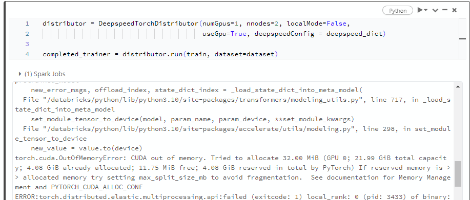
To limit the chance of this happening, we recommend following these steps to establish an optimal configuration:
- Estimate your memory requirements using the table above
- For model precision, use bfloat16
- For optimizer and gradient settings, use ZeRo 3
Try a training run and see how it goes. If you find yourself running into out-of-memory issues, progressively add offload and set gradient accumulation steps and turn on gradient checkpointing. The training process may run more slowly, but it will be more likely to complete.
Monitoring and debugging
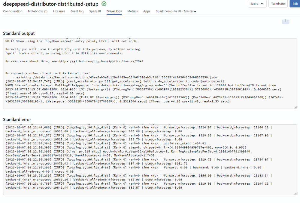
The best way to monitor and debug DeepSpeed training runs is to look at the Metrics and Driver logs tabs in the Databricks web UI:
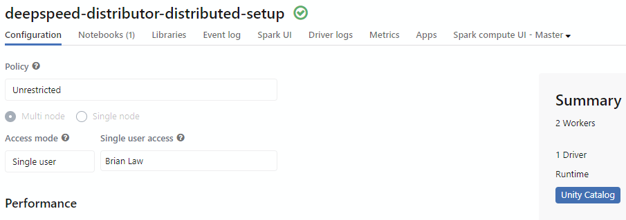
The metrics tab has separate dropdowns for hardware settings, including GPU and CPU utilization. 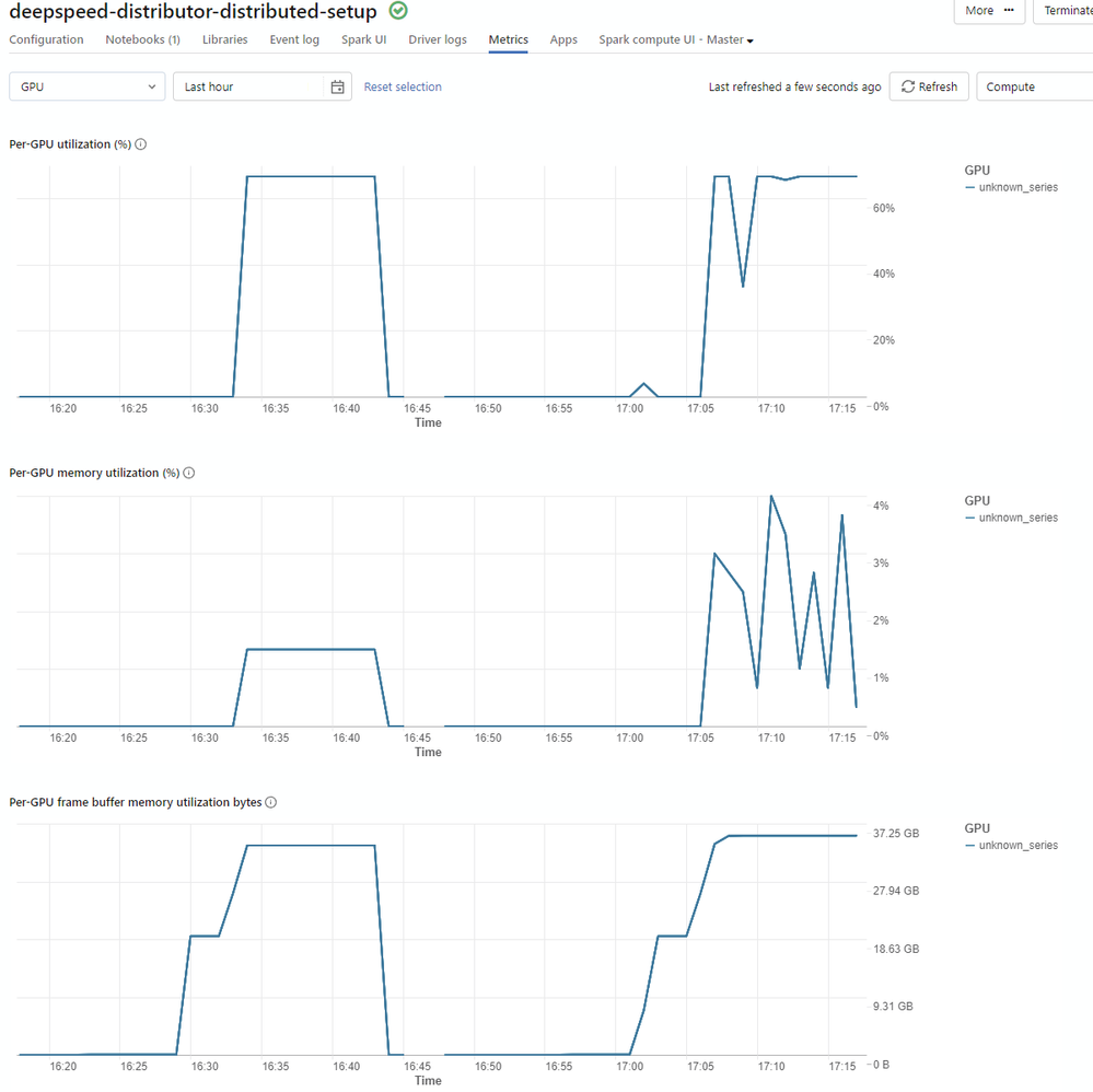
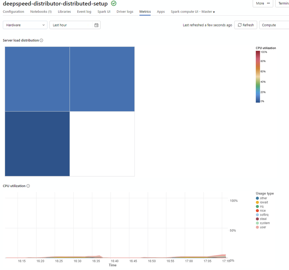
The driver logs will give us the same debug details that would appear in a terminal session should the excerpts displayed in the notebook prove insufficient.
Conclusion
The DeepSpeed Distributor on Databricks marks a pivotal advancement in efficiently training large language models by significantly reducing GPU memory requirements. It simplifies resource configurations and management, enabling scalable and optimized AI project development. Try it out on Databricks today using the code found here.
1 Comment
You must be a registered user to add a comment. If you've already registered, sign in. Otherwise, register and sign in.
Related Content
- The next generation of Databricks Genie in Announcements
- 🌟 Community Pulse: Your Weekly Roundup! April 20 – 26, 2026 in Announcements
- 🌟 Community Pulse: Your Weekly Roundup! April 06 – 12, 2026 in Announcements
- Agent Bricks | A Pilot to Production Series 🚀 in Databricks TV
- Intelligence Studio -- Open-Source AI-Powered API Explorer for Databricks in Community Articles
